💡
N hidden layers Neural network = Deep Learning
Function with unknown → Define loss from training data → Optimization
y=fθ(x) → L(θ) → θ∗=argminL(θ)
Regression
The function outputs a scalar
Model → y=b+wx1 (linear model)
Model → y=b+∑wx1 (increase domain knowledge)

Classification
The function outputs a correct given options(classes)

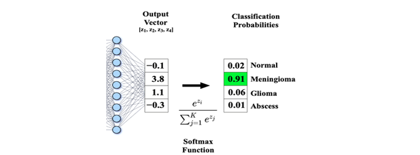
Softmax
y′=softmax(y) (Normalize y to 0 < y′ < 1)
y′=j∑exp(yi)exp(yi)
j∑yi′=1


Minimize cross-entropy == maximize likelihood
softmax == 2 input sigmoid
Loss
A function of parameters. How good a set of value is.
yˆ → label
ei=∣yi−yˆi∣ → Mean Absolute Error
ei=(yi−yˆi)2 → Mean Square Error
L(b,w)=N1∑ei → loss(small the best)
Optimization
Gradient Descent
θ∗=minL(θ)
η → learning rate. (hyperparameter)
ηδθδL → Gradient Descent(only find local minima)
θ1=θ0−ηδθδL∣θ=θ0 (reverse direction of gradient)
g=∇L(θ0)
If gradient is negative, increase θ.
θ1=θ0−ηg
Hyperparameter: defined by ourselves.
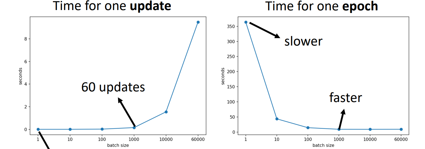
epoch = N × Batch Updates
Critical points

Find loss function near θ=θ′
Tayler series approximation
L(θ)≈L(θ′)+(θ−θ′)Tg+21(θ−θ′)TH(θ−θ′)
L(θ)≈L(θ′)+vTg+21vTHv

Local minima
vTHv<0, for all v
H is positive defined → All eigen values are positive

Local maxima
vTHv>0, for all v
H is negative defined → All eigen values are negative

Saddle point
else

uTHu = uT(λu) = λ∣∣u∣∣2
θ−θ′=u θ=θ′+u
Update direction: (λi<0)→ui
💡
Eigen value
λ →
det(A−λI)=0Eigen vector
ui →
(A−λiI)ui=0
Batch (a hyperparameter)
epoch = see all batches once → shuffle after each epoch(divide to batches)
- Batch size = N (full batch)
- Batch size = 1
- Noise is better for training & testing
For parallel computing

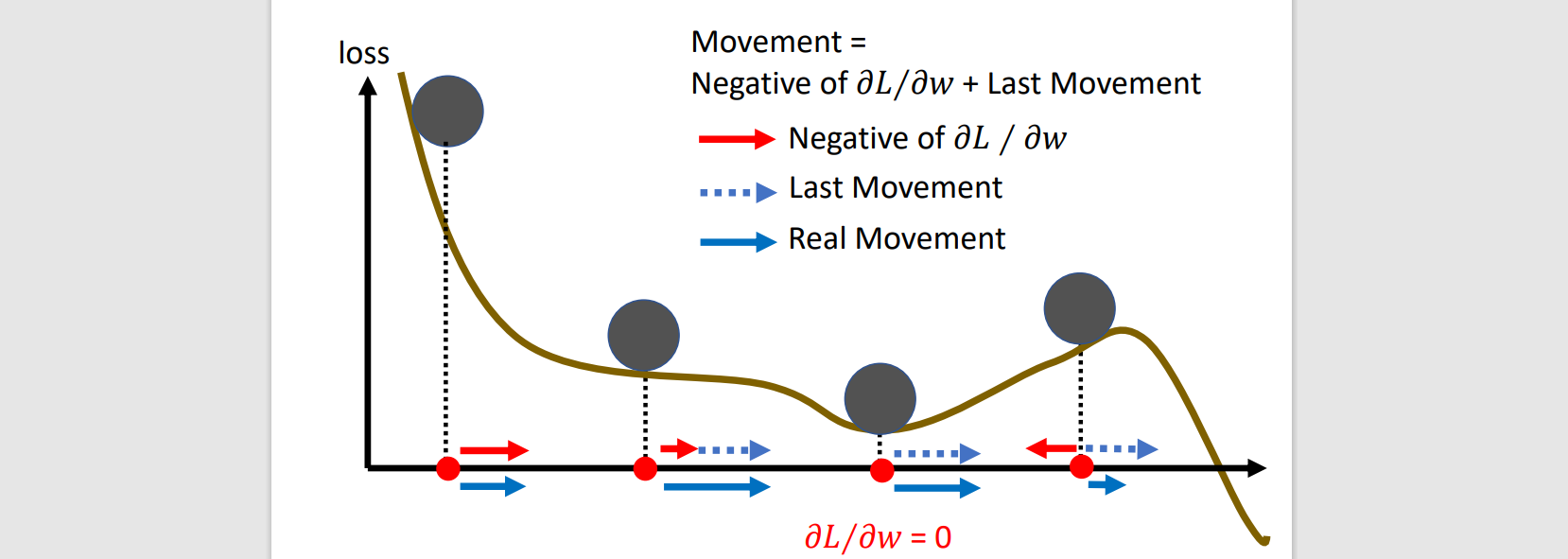
Momentum
Mimic real world physics

Movement(m): movement of last step - gradient at present, m0=0
m1=λm0−ηg0 (movement) → (sum of all past gradients)
θ1=θ0+m1 (move to)

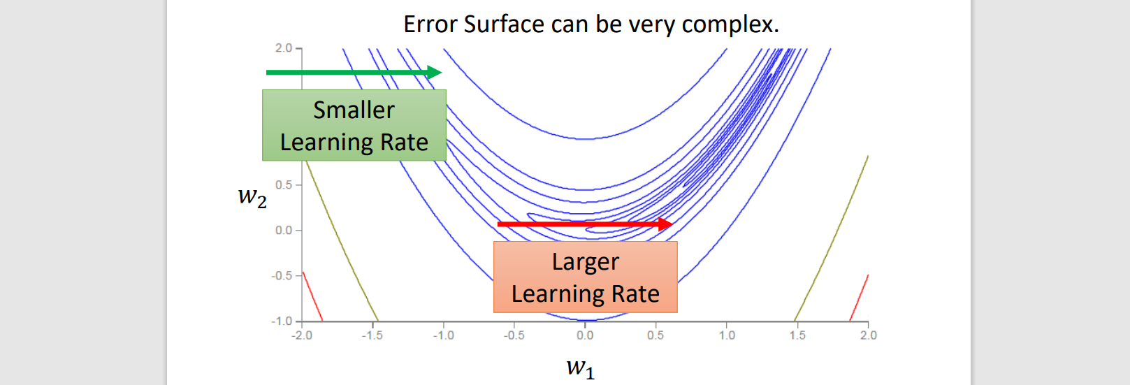
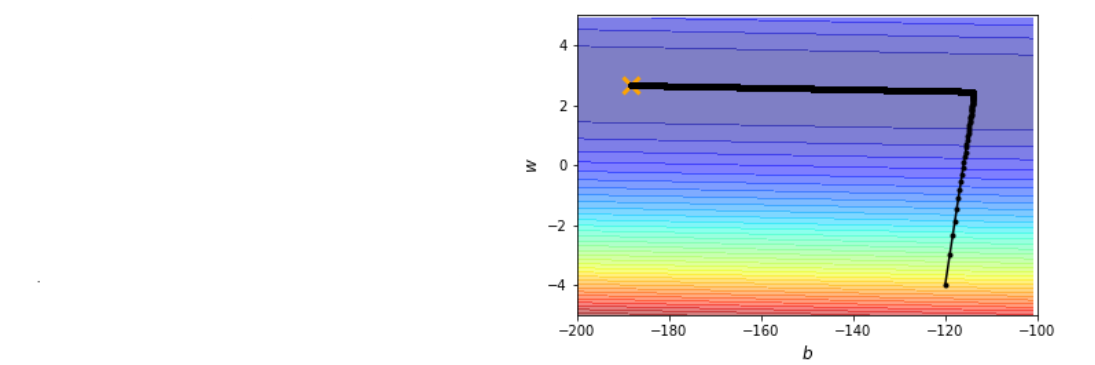
Adaptive learning rate
θit+1=θit−σitηgit (parameter/time dependent)
Root mean square
σit=N1t=0∑N−1git
If g is big → decrease η

RMSProp
σit=α(σit−1)2+(1−α)(git)2
0<α<1 (decide the importance of previous α)
Small α → fast reaction to new g
Adam
RMSProp + Momentum
θit+1=θit−σitηtmit
ηt → scheduled η
m → previous direction of g
σ → previous magnitude of g
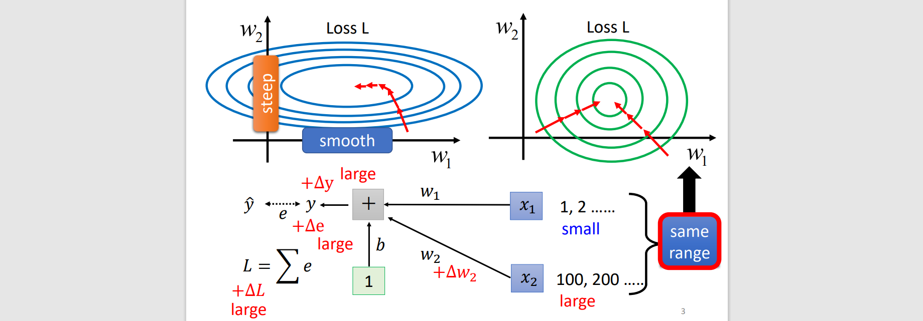
Batch Normalization
Smooth error surface

wi+Δwi→L+ΔL
large xi has greater affect

Feature normalization

If desired output ≠ 0 → add network parameter
xˆi=γ⊙x˜i+β
- ⊙ → element wise multiplication
- γ → initially a 1 vector (until a good error surface is found)
- β → initially a 0 vector (until a good error surface is found)
Testing stage
Moving average of training
x˜ir=σˉixir−μˉi
μˉ=pμˉ+(1−p)μt
Models
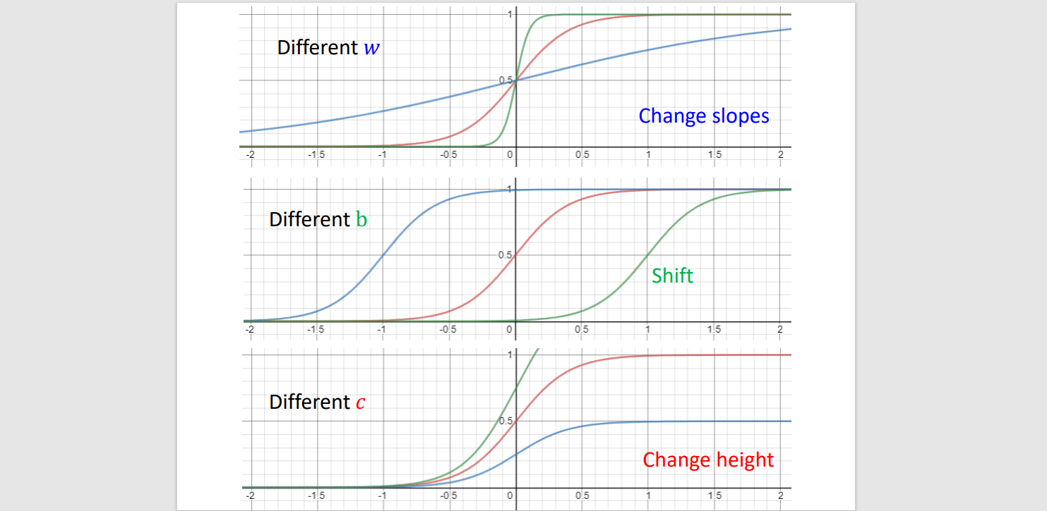
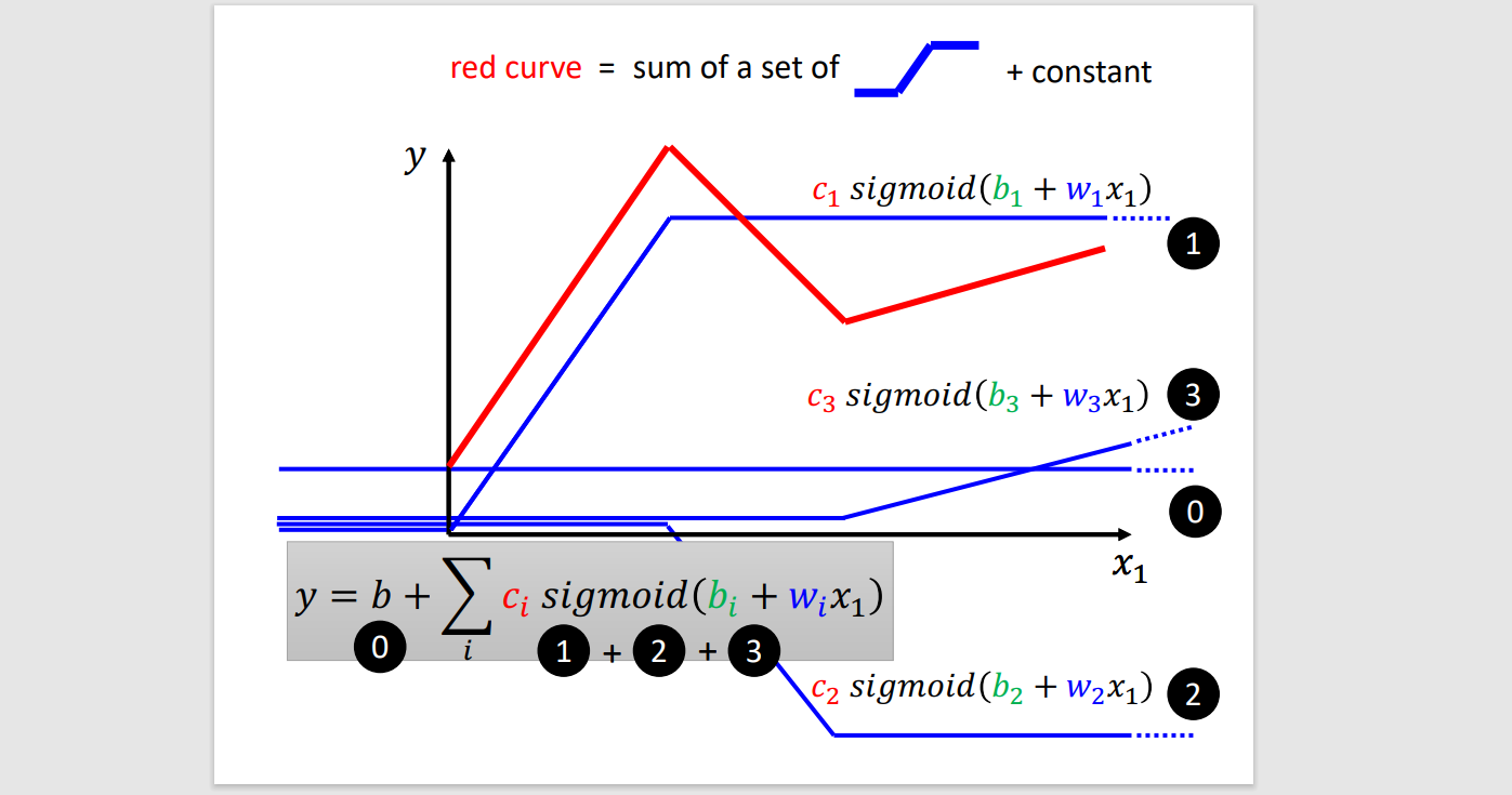
- Piecewise Linear - sets of sigmoid(activation) functions {Neuron}
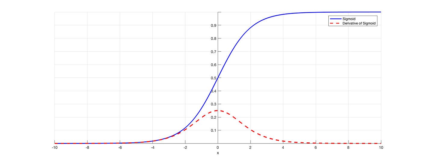
yn=c⋅sigmoid(b+wxi)=c1+e−b+wxn1

yn=b+∑ci⋅sigmoid(bi+wixn)

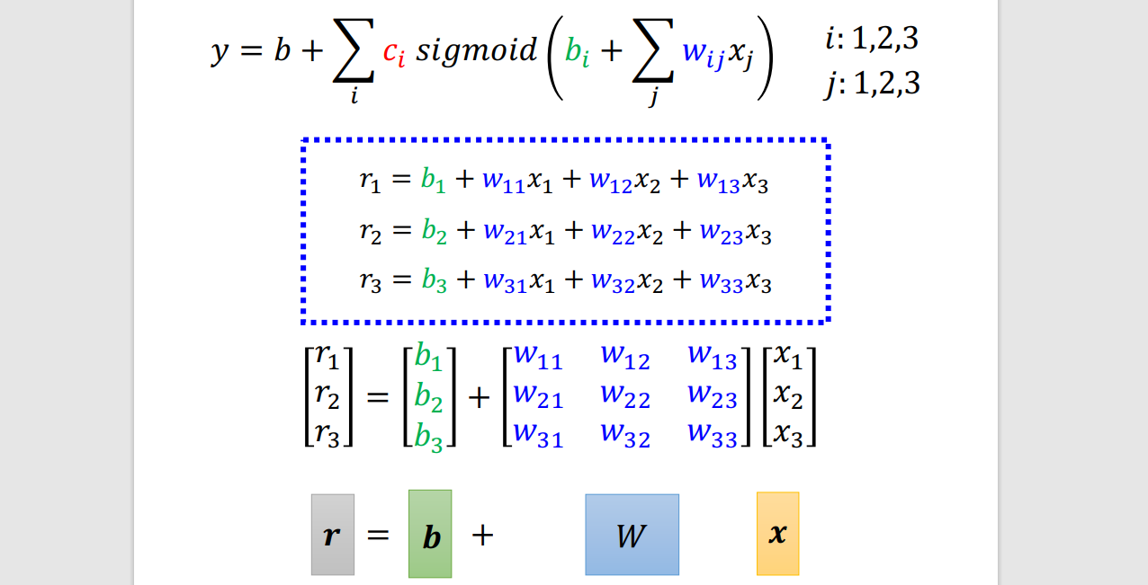
yn=b+i∑ci⋅sigmoid(bi+j∑wijxj)
- i → piecewise sigmoid function
- j → range of knowledge domain
Linear Algebra
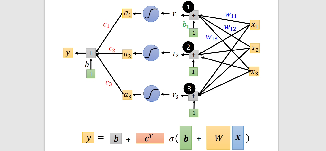
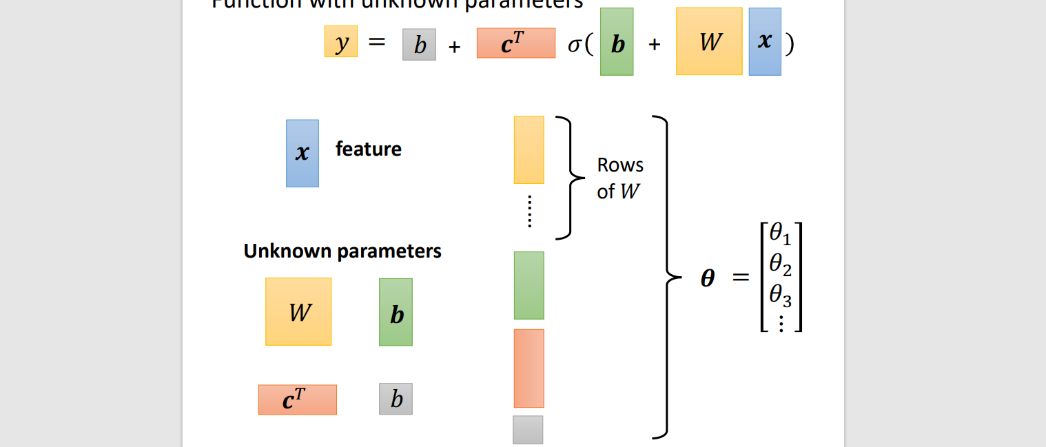
1 layer


Feature: x
Unknown parameter (θ): y,b,cT,w

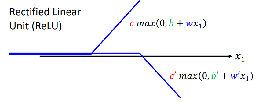
Rectified Linear Unit(ReLU)
yn=b+i∑ci⋅sigmoid(bi+j∑wijxj)

yn=b+2i∑ci⋅max(0,bi+j∑wijxj) → ReLU (better)

- Overfitting → Good training data, bad unseen data.
Backpropagation
An efficient Gradient Descent
Chain Rule
y=g(x)z=h(y)
dxdz=dydzdxdy
Δx→Δy→Δz
x=g(s)y=h(s)z=k(x,y)
dsdz=δxδzdsdx+δyδzdsdy
Δs Δz
Cn → distance between yn & yˆn
L(θ)=n=1∑NCn(θ)
δwδL(θ)=n=1∑NδwδCn(θ)
δwδC=δwδzδzδC
- Backward pass
δzδC=δzδaδaδC
a=σ(z) activation function

δaδC=δaδz’δz’δC+δaδz’’δz’’δC
δaδz’=w
δzδC=σ’(z)[w3δz’δC+w4δz’’δC]
σ’(z) is a constant
δz’δC=δz’δy1δy1δC δz’’δC=δz’’δy2δy2δC
Improve training
Observe training data first, then testing data.
Model bias
y=b+wx1
- More features: increase domain knowledge y=b+∑wx1
- More layers: deep learning yn=b+i∑ci⋅sigmoid(bi+j∑wijxj)
Bad optimization
Big training data loss
- Gain insight from shallow network optimization
- Data augmentation(隆乳): generate new data from existing data
- Constrained model: based on our interpretation of the problem
💡
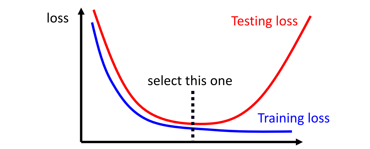
Overfitting:
Small training data loss + Big testing data loss
optimization not enough, higher layer must be better

Mismatch
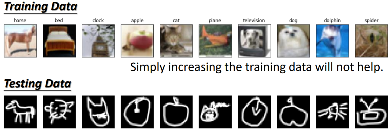
Distribution of training & testing data is different
